New paper in SMR: A Method for Studying Difference in Segregation Levels Across Time and Space
Benjamin Elbers. A Method for Studying Difference in Segregation Levels Across Time and Space. Sociological Methods and Research.
The Problem: Margin dependency
An important topic in the study of segregation are comparisons across space and time. It has been recognized for a long time that many segregation indices are margin-dependent, which complicates such comparisons. For instance, it can be shown that the index of dissimilarity (\(D\)) is margin-dependent in terms of the units under study (e.g., neighborhoods or schools), but not in terms of the groups (e.g., racial/income groups). This led to a debate in the gender segregation literature in the 1990s, where Charles and Grusky (AJS 1995, Demography 1998) advocated the use of log-linear modeling.
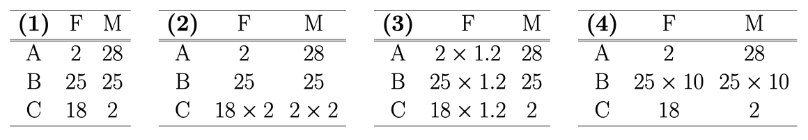
Consider the following four tables, which cross-classify the number of male and female employees across the occupations A, B, and C. Table (1) shows the baseline situation. In Table (2), occupation C has grown, while in Table (3) female employment increased across all occupations. Table (4) shows an extreme example, where the integrated occupation B has grown strongly.
How do different segregation measures characterize these situations? The following table shows how the popular \(D\), \(M\), and \(H\) indices, as well as Charles and Grusky log-linear index \(A\), quantify the amount of segregation. Also shown are the two odds ratios \((F_{A}/M_{A})/(F_{B}/M_{B})\) and \((F_{C}/M_{C})/(F_{B}/M_{B})\).
| Table | \(D\) | \(M\) | \(H\) | \(A\) | Odds ratios |
|---|---|---|---|---|---|
| (1) | 0.465 | 0.203 | 0.295 | 7.22 | 0.0714 and 9 |
| (2) | 0.501 | 0.233 | 0.337 | 7.22 | 0.0714 and 9 |
| (3) | 0.465 | 0.206 | 0.297 | 7.22 | 0.0714 and 9 |
| (4) | 0.001 | 0.000 | 0.000 | 7.22 | 0.0714 and 9 |
The indices \(D\), \(M\), and \(H\) are margin-dependent in either one or both directions, while the log-linear indices and the odds ratios stay stable. However, they also do stay stable in the extreme example, which many would regard as not very segregated.
I make use of the M index, which is margin-dependent in both directions, can be standardized (H index), and is highly decomposable:
\[ M =\sum_{u}p_{\cdot u}\text{L}_{u}\text{ where }\text{L}_{u}=\sum_{g}p_{g|u}\log\frac{p_{g|u}}{p_{g\cdot}} \]
Defined for a \(U \times G\) contingency table, where \(u\) indexes the units, and \(g\) the groups; where \(p_{\cdot u}\) (\(p_{g \cdot}\)) is the marginal probability of being in unit \(u\) (group \(g\)); and where \(p_{g|u}\) is the probability of being in group \(g\) given unit \(u\). \({L}_{u}\) is called the local segregation score for unit \(u\).
The Solution: Decomposition of \(M\)
To decompose the difference between two \(M\) indices at times \(t_{1}\) and \(t_{2}\) into marginal and structural components, we construct two counterfactual matrices:
- \(t'_{1}\), which has the same marginal distributions as \(t_{2}\), but the odds ratios from \(t_{1}\),
- \(t'_{2}\), which has the same marginal distributions as \(t_{1}\), but the odds ratios from \(t_{2}\).
This allows for the following decomposition:
\[ \begin{aligned} M(t_{2})-M(t_{1}) & =\overbrace{\frac{1}{2}(M(t_{2})-M(t'_{2}))+\frac{1}{2}(M(t'_{1})-M(t_{1}))}^{\Delta_{\text{marginal}}}\\ & +\underbrace{\frac{1}{2}(M(t_{2})-M(t'_{1}))+\frac{1}{2}(M(t'_{2})-M(t_{1}))}_{\Delta_{\text{structural}}} \end{aligned} \]
To construct the two counterfactual matrices, we use Iterative Proportional Fitting (IPF). To construct \(t'_{1}\), take \(t_{1}\) and adjust all cells towards the column marginals of \(t_{2}\). Then adjust all cells towards the row marginals of \(t_{2}\). This adjustment towards the column and row marginals is repeated until both marginals have converged, i.e. are similar to those of \(t_{2}\).
There are a few straightforward extensions of this decomposition:
- Decomposition of \(\Delta\)marginal. It is often of interest to determine how much the row and column marginals have contributed to segregation change separately. To decompose the marginal component further, define \(M(U;G;O)\) to identify the \(M\) that is calculated based on the unit marginals from \(U\), the group marginals from \(G\), and the odds ratios from \(O\).
\[ \begin{aligned} \Delta_{\text{marginal-units}} & =\frac{1}{4}(M(t_{2};t_{1};t_{1})-M(t_{1};t_{1};t_{1}))+\frac{1}{4}(M(t_{2};t_{2};t_{1})-M(t_{1};t_{2};t_{1}))\\ & +\frac{1}{4}(M(t_{2};t_{2};t_{2})-M(t_{1};t_{2};t_{2}))+\frac{1}{4}(M(t_{2};t_{1};t_{2})-M(t_{1};t_{1};t_{2}))\\ \Delta_{\text{marginal-groups}} & =\frac{1}{4}(M(t_{1};t_{2};t_{1})-M(t_{1};t_{1};t_{1}))+\frac{1}{4}(M(t_{2};t_{2};t_{1})-M(t_{2};t_{1};t_{1}))\\ & +\frac{1}{4}(M(t_{2};t_{2};t_{2})-M(t_{2};t_{1};t_{2}))+\frac{1}{4}(M(t_{1};t_{2};t_{2})-M(t_{1};t_{1};t_{2})) \end{aligned} \]
This procedure requires six IPF procedures in total, and is based upon the elimination of the marginal contributions in all possible ways (Shapley value decomposition).
- Decomposition of \(\Delta\)structural. It is also possible to decompose structural change into the contributions of each individual unit by exploiting the decomposability properties of the \(M\) index:
\[ \begin{aligned} \Delta_{\text{structural}} & =\frac{1}{2}(M(t_{2})-M(t'_{1}))+\frac{1}{2}(M(t'_{2})-M(t_{1}))\\ & =\sum_{u}\frac{1}{2}\left(p_{\cdot u}^{t_{2}}\left[L_{u}(t_{2})-L_{u}(t'_{1})\right]+p_{\cdot u}^{t_{1}}\left[L_{u}(t'_{2})-L_{u}(t_{1})\right]\right) \end{aligned} \]
- (Dis)appearing units. In many segregation problems, the researcher has to deal with units that disappear over time, or new units that appear. For instance, in a school segregation problem, schools may close down and new schools may open up. It can be shown that the \(M\) index provides a clear interpretation for the contribution of these (dis)appearing units towards segregation.
Example: Occupational Gender Segregation
I now apply the full decomposition to the study of occupational gender segregation of the civilian population of the United States between 1990 and 2016:
\[ \begin{aligned} M(t_{2})-M(t_{1}) & = \Delta_{\text{additions}} + \Delta_{\text{removals}}\\ & + \Delta_{\text{marginal-units}} + \Delta_{\text{marginal-groups}}\\ & + \Delta_{\text{structural}} \end{aligned} \]
The data source is the U.S. Census and the American Community Survey, downloaded from IPUMS. Harmonized occupational codings come from IPUMS. Some 50 occupations vanish over time, but no new occupations are introduced. The decomposition was carried out for the whole population, as well as for 9 major occupational groups separately.

The figure shows that:
- overall gender segregation has been declining,
- much of this is due to changes in the structural component, i.e. the odds ratios,
- disappearing occupations do not matter very much, except for operators/laborers,
- there is some heterogeneity by major group: declines have been pronounced in some groups, but in some major groups gender segregation has increased,
- much of the decline in segregation is structural, while the increase is mostly due to marginal changes,
- the three components can offset each other.
See also the R package segregation which accompanies this paper.